Google Colaboratory or Google Colab is an online notebook that allows coding and writing Python in the browser. 

It is equipped with various Machine Learning libraries, and it can harness the full potential of Python libraries. Scientists and engineers take advantage of its broad capabilities.

It’s free

Google Colab is always free to use. All features are also accessible to a certain degree. The upgraded features, though, can be accessed through the Google Colab Pro subscription plan at a rate of  $9.99 per month in the following countries:

• Brazil
• Canada
• France
• Germany
• India
• Japan
• Thailand
• UK
• US

Advantages of using Google Colab

• Free to use – anyone can access 
• Easy start – getting started is easy
• Can access GPUs/TPUs – it is ready and fully equipped for a great coding environment
• Codes can be shared with others – easy sharing is done with Google Drive and direct to GitHub as well
• Graphical visualization is easy in Notebooks – coding in blocks and multiple graphical displays

Disadvantages of using Google Colab

• Limited usage of GPU/TPU – GPU/TPU in the free version is good only for 12 hours
• Not powerful – Other setups are more powerful in terms of GPU/TPU  
• Not the best in de-bugging – De-bugging environment is not reliable
• Limited data space – Not capable of handling big data
• Re-install of several dependencies is necessary – additional libraries should be re-installed from time to time

Alternatives to Google Colab

There are other platforms that can be used instead of Google Colab. Some are even more suitable to specific needs. The following are some of them:

• Amazon SageMaker
• Azure Notebook
• FloydHub
• Jupyter Notebook
• Kaggle
• Paperspace Gradient

Google Colab in supporting Python

Google Colab is focused on supporting Python and other tools. However, as of October 2019, it only allows the Python 3 notebook creation. In January 2020, Google Colad no longer supports Python 2.

Getting started with Google Colab

Getting started with Google Colab can be done in several ways. Each approach is easy, depending on what is needed to accomplish.

Approach 1: Google Drive

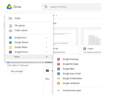
In using Google Drive, select “New” at the upper left corner and click “More.” From the drop-down panel display, choose “Google Collaboratory”.

To open a document in Google Colab, click the  “–> Open With –> Google Collaboratory”. If you share Google Drive with others, they can open your documents and you can also open theirs through Google Colab.

Approach 2: GitHub

To directly import or open documents from GitHub with Google Colab,  use the chrome extension “Open in Colab”.  Add the extension to your chrome, and then, open the notebook. In the Extensions tab of your chrome, select “Open in Colab.”

Give it some time to polish up in your browser before using it in your Google Colab documents. 

Approach 3: New Notebook

To go to the new notebook link, click “New Notebook”.

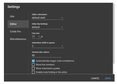
There are also a lot of things that you can do when you open a New Notebook in Google Colab. Aside from naming your document, you can also change some of the settings as desired.

On the Settings page, you can customize the color, font size, and the like according to your preference.

Here are some of the useful control commands:

• Press Ctrl+Alt+M to add a comment
• Press Ctrl+B B  to add a cell below 
• Press Ctrl+Shift+P to command pallete 
• Press Ctrl+M M  to convert to text cell 
• Press Ctrl+F9 to run all cells 
• Press Ctrl+Enter  to run the current cell 
• Press Ctrl+S  to save a Notebook
• Press Ctrl+M H  to show the keyboard shortcuts 

Keep in mind that all those shortcuts are editable to suit your preference and needs.

As shown in the image below, the left taskbar displays the table of contents of your Notebook. There are also the Markdown headers, files, code snippets, and search and replace tools.

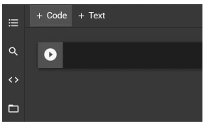
In the upper right of the screen, look for the connect button. Click it and start coding. Here’s what you will see:

So this is the Google Colab and some of its main features. It’s time to test it by starting with a new problem to work on.

Importing libraries and installing dependencies in Google Colab

Using Google Colab is easy, and the needed import/install of dependencies is simple. The commands “!pip install” and “import” will be used here, together with the name of the libraries. 

Meanwhile, there are different preinstalled libraries in Google Colab, and they are just good to use anytime.

However, most of the installations added to these preinstalled files may need reinstallation on the next project once the session is closed. 

It is a good move to check on the library to know the version you are currently using. To do this, type “!pip show” followed by the name of the tool you want to check. 

If you want to upgrade to the latest version, type “!pip install –upgrade” followed by the name of the tool.

You can also install a version that you think suited your needs most. Type “!pip install” followed by the  tool’s name and version.

Enabling usage of GPU/TPU in Google Colab

In the Notebook Settings, go to the “Runtime” section and click the “Change runtime type” and GPU to TPU to enable its usage.

The Google Colab documents allow the utilization of TPU’s full potential. Most of these features can be accessed and utilized in the “TPUs in Colab”.

Importing data in Google Colab

Importing data in the Google Colab direct from Google Drive is so simple. You can use the PyDrive and REST API for this action. It includes mounting of drive in the Notebook.

To mount the Google Drive, this link is useful. It will help you with the methods, how to use them and how to go over them. 

Follow this code for this action:

A coded output is necessary to authorize the action. You can get that through the link shown in the image below:

This link will prompt you to this screen:

Copy the authorization code that will appear on your screen and paste it into the blank cell. Press “Enter” to access it.

Other things that you can do with your drive include opening a text document, writing texts, and saving the document. Here’s how:

Most of the data for machine learning work are “csv” and “xlsx” files and are loaded to pandas data frames. Image data are also loaded into arrays. With Google Colab, this is done as simply as it can be.

Assuming the drive is already mounted in the same way shown above. Through Google Drive, simply upload the “csv/xlsx” file. You will see that the location of the file has a path of “/content/drive/My Drive/”. The file you uploaded and saved has a path of “/content/drive/My Drive/Name”.

To load your file directly from pandas to the pandas data frame, use the “read_csv” function like the image shown below:

To directly upload the file from the computer, follow the codes shown in the image below:

To open the files you want to open and read, click “Choose Files.”

Finally, to stream the data through the pandas data frame, the BytesIO function will be used. 

In the examples given below, most of the datasets are from Kaggle. You can directly open it in Google Colab and there is no need to download the files.

Predicting House Prices Using Machine Learning in Google Colab

The goal of creating a Google Colab machine learning algorithm is to predict house prices in the future. To reach this goal, you will need to use the California House dataset. Here is the link for this dataset:

https://www.kaggle.com/datasets/camnugent/california-housing-prices

Direct Loading of Kaggle datasets into Google Colab

Kaggle, which has  API clients of its own, enables users to directly load and get the datasets into their notebooks. For Google Colab, this is how it is done.

As shown in the image below, a Kaggle API token was created. First, you will go to your account in Kaggle, scroll down the details, and look for the API section. In the said section, click “Create New API Token”. This will prompt you to a screen showing that a Kaggle JSON file is being downloaded.

Your next step is to import the libraries to your notebook to start loading the dataset. Check this image:

Then check if the Kaggle.json file you downloaded is correct and saved in the right location. Check the image for referrence:

After the files are located, it’s time to set the configuration. See the image below:

The dataset is now ready to be downloaded from Kaggle. On your Kaggle dataset, copy this API command just as how it is shown in the image below:

Paste this command and wait for Google Colab to download it. Follow the command in this image:

Open the downloaded file. Unzip and remove the zip with this command:

On the left corner of the page is the toolbar. You will find the Files icon here and see the housing dataset that you unzipped from the downloaded file.

Look at the dataset as shown in the image below:

Visualizing the data or producing charts using Google Colab

Google Colab and Jupyter Notebooks have similarities. After the graphing command is run,  you will see the graphs instantly. These graphing libraries are mostly ggplot, matplotlib, plotly, and seaborn.

The dataset is now ready to be explored. You can do it by making a thorough EDA or Explanatory Data Analysis. Take a look at this image of a dataset with all the values included.

In the dataset shown above, notice the values of each item. The variable of “total_bedrooms” is different from the variables of the rest of the items in the dataset. It means that there are missing values in total_bedrooms. The ‘Dtype’ value of “ocean_proximity” is 1, and it is noticeably different as well. Later in the discussion, this matter will be explained. For now, take a look at the images below:

Furthermore, the pandas “describe” function is useful in  describing the variables as shown in the image:

For the graph of these variables, you will be using the matplotlib. Look at the histogram first. Here is the image:

Based on the graph shown above, you can see that the “median_income” histogram values were already preprocessed and scaled. You will clearly observe that the expression of numbers is in tens of thousands in US dollars. 

The skew distribution, which leans more on the left side, is also visible in the graph shown above. The variables appear in different scales, and it is one of the topics that need further discussion. 

Take this helpful tip: Data snooping uses data mining inappropriately and it leads to biased results. To avoid Data Snooping Bias, later on, make sure to split the data into two sets before doing the EDA. Separate the train set from the test set. 

In this example, the data is split with a twist into the train set and test set. As discussed above, the median income predicts the house value better than other approaches. This is why the data represents the median income stratums. 

Based on the median income histogram, the data is mostly between 1.5 and 6. But the data can go even beyond 6 at some time. If there are not enough instances in a set, biased data can be the result.

It can be avoided by simply using the “pd.cut” function. Look at the images below:

The next step to take is to split the data into stratums and then remove them. Check the image below:

Then change the graph so that it shows the housing prices. You will notice that the population in the district is represented by the radius around the circle. Also, the color in the graph represents the price.

The graph above shows that the Bay Area, also the area in San Diego, and in Los Angeles are among the areas with high density. The Central Valley and around the areas of Fresno and Sacramento also have some density.

As expected, the density in the graph is related to housing prices. It shows that the houses located in proximity to the sea are being sold for a higher price. Check these images for the correlations.

Keep in mind that the features should make sense or that they are more informative. To do that, you need to make a correlation matrix.

To illustrate the correlation matrix, the image shows that three features are combined to give further information. Notice how they are created. There are data for bedrooms in a room, rooms for each household, and population in a household.

There is a noticeable correlation between the “room_per_household” with label compared with the “total_rooms” and ”households”. Meanwhile, the “bedrooms_per_room” also shows a correlation with the label and not with its parent variables.

The simple interpretation of the data shown is that when the median income shows a higher numerical, it means that the house prices are higher. Also, when the ratio of bedrooms per room is low, it means that the prices are getting higher.

Look at the image below to see the correlation of the top 4 variables and how they are correlated with each other:

The image above shows the behavior of variables with other variables. The median_income and median_house_value also show that house prices are mostly valued at $500k.

Deploying Machine Learning Algorithms in Google Colab

Machine Learning or ML algorithms are used in Google Colab just as how they are used in various coding environments. These preinstalled ML libraries, along with the scikit-learn and TensorFlow are important features of Google Colab as well.

3 Steps to deploying ML Algorithms:

1. Preparation of Data

Before any deployment of any ML models, the first step is always data preparation. You need to prepare the data, preprocess it, and make it ready for the algorithm. 

In the data shown, most of the features are numerical. But there is one feature that is categorical, and that is the “ocean_proximity”. Different features are prepared and preprocessed differently. 

The first part of the preparation of data is to split the train set into two and one of those contains the label.

In preparing the data, the usual process is to automate it by splitting the “housing_features” into categorical and numerical. Then the functions and sklearn pipelines are created before proceeding to the process.

The sklearn numerical pipeline that you will create is one that:

• Makes new features
• Adds the missing data 
• Standardizes the numerical features

It means that the goal is to import the libraries or dependencies and, at the same time, to customize a function to be used in creating new features. Keep in mind that such a function allows for choosing the right features.

It’s time to create a numerical pipeline:

After creating a numerical pipeline, you will then create the categorical pipeline. This one performs the One Hot Encoding for the “ocean_proximity” feature. These two different pipelines are then combined into one pipeline that will run the features.

2. Picking and Evaluation of an Algorithm

The best move in doing machine learning is to pick several algorithms which can be compared with each other. From the compared algorithms, you will pick the best one to evaluate. 

In this article, the best pick is the Random Forest Regressor. You can do some practice with this data by building multiple algorithm pipelines, and then compare them, and finally, get a copy of the comparisons. 

Part of the step is to check the RMSE. It shows the difference between observed values and predicted ones.

3. Optimization of the Algorithm

Optimizing the ML algorithm is done by performing a random search for hyperparameters. The goal of specific searching is to look for the optimal ones because they are going to be used as models.

In this image, you can see that there are hyperparameters with low values. Try to look for errors.

The image above displays a dataset of 189 estimators at a max of 8 features.

Directly Saving My Google Colab Notebook to GitHub

Google Colab Notebook can be directly saved to GitHub. This is done by going to the “File” section of the Google Colab notebook and then clicking “Save a copy in GitHub”. A screen that asks for an authorization code will then pop-up.

Mounting External Python Files in Google Colab

For the external python files or code in your  Google Drive, you can opt to run the files with their GPU or TPU in the Google Colab. Here is the command:

After writing the command, a URL is given to take you to the tab that permits access to Google Drive. Enter in the code cell the authorization code that appears.

Here is the command that you will need to write to allow a specific content to run in the drive:

Another command to write is the following. This is to run specific file or content in the drive.

Google Colab Magics

Google Colab magics are some system commands that are also considered an extensive command language. Line Magics and Cell Magics are the two types of Google Colab Magics.

To compare these two magics, the line magics always have the “%” at the beginning, while the cell magics have the “%%” at the start. Check and see the full list of these magics by typing the following command:

To show the local directory using the line magic, this is what to write in the commands:

For the cell magic, this is the command to write:

Other Interesting Features of Google Colab

Google Colab offers a wide variety of interesting features. These features include a markdown for mathematical equations, forms, custom widgets, and a lot more. Check this link for more Google Colab features: https://colab.research.google.com/notebooks/intro.ipynb

3 Common Mistakes in Machine Learning Analysis/Testing

Take note of these common mistakes in running the analysis/testing:

• Look-ahead Bias
• P-hacking
• Overfitting

want to learn how to algo trade so you can remove all emotions from trading and automate it 100%? click below to join the free discord and then join the bootcamp to get started today.