If you are interested in Linear Regression, this article will show you a step-by-step guide on how to implement linear regression in Python.

What is Regression Analysis?

It is a statistical method used in finance to determine the relationship between variables – how important they are and how they affect each other. 

There are two variables – dependent and independent variables. Dependent variables are the variables were are trying to predict or understand. Independent variables, on the other hand, are independent factors that may affect or influence the dependent variable.

What is Linear Regression?

Linear regression specifically refers to the statistical method for modeling linear relationships between variables. A simple linear regression predicts the response variable with one explanatory variable, while a multiple linear regression predicts several explanatory variables.

When do you use Linear Regression?

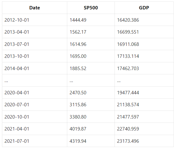
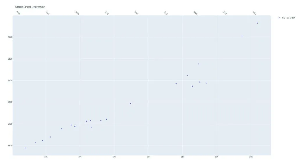
We use linear regression when there is a linear relationship. An example is a relationship between the S&P 500 index price and the GDP. In essence, the stock prices go up as the companies sell more goods.

Let’s explore if it is true in this example:

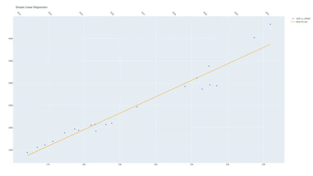
The straight line in the chart is called the regression line.

Determining Best Fit Line (OLS)

Ordinary least squares (OLS) is a linear least squares method used to estimate unknown model parameters.

In drawing a straight line, remember this linear equation:

y = mx + b

So, in the example, we have the following:

• y is the S&P500 price or the value we want to predict
• x is the GDP
• m and b are model parameters that we’re trying to fit

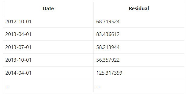
When we say fit, we estimate the values that make the best fit line by minimizing the error, which is the difference between the GDP vs. SP500 points (actual) to the best fit line (prediction).

The OLS takes the difference and then adds them to get the squared error. Here is the equation:

SquareError = (a-p)^2 + (a_2-p_2)^2 …

• a is the actual
• p is the predicted

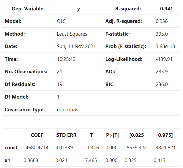
We find the line that minimizes the squared residuals. Here’s an example of the OLS regression results for clarity:

The issue with squared error is that more points will lead to a higher squared error even if the line fits better. To fix this, we get the MSE or mean squared error.

To get a meaningful number, we get the square of the above number.

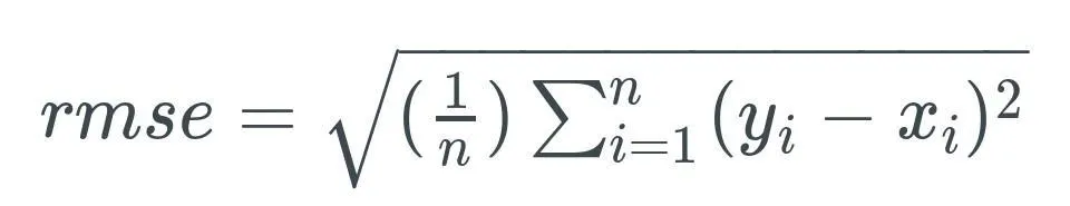
With the RMSE, two issues are addressed:

• make the differences positive
• punish increasingly poor prediction

So, what’s the formula for our best fit line? Let’s look at this:

If you said:

y = mx + b s&p500 = m *gdp + b * y_hat = 0.3688gdp + -4680.4714

You would be correct.

Also, as we’ll use it later on, we can rearrange the formula and turn m into a b:

y = mx + b to y = b_0 + b_1 * X_1

• y or “Y hat” simply means it’s a predicted or expected variable
•  X’s are the independent variables
• B’s are the regression coefficients

In summary, for every unit of GDP, we expect to add 0.3688 points to the S&P500. If the GDP is zero, the S&P500 is predicted to be -4680.4714.

Polynomial Regression

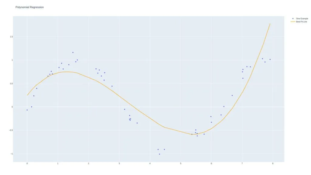
We use polynomial regression if the regression line does not fit the model. We can use exponential formulas such as the following to model our relationships.

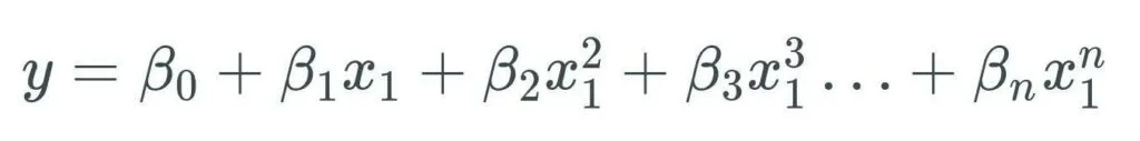
Here’s a third-degree polynomial regression model:

Understanding Regression Performance

In this section, we will discuss r-squared (r2). It is the proportion of the variation explained by the predictor variables in the observed data. The higher the r-squared, the better.

In our example, the r2 is 0.941, which means that 94% of the observed data can be explained using our formula, and the other 6% cannot. The high r2 means that the predictor variables predict the dependent variables from the historical data quite well.

Simple Linear Regression in Python

Let’s perform a regression analysis on the money supply and the S&P 500 price.

Here are the three different ways in which the Federal Reserve  controls the supply of money:

• Reserve ratios – How much of their deposits banks can lend out
• Discount rate – The rate banks can borrow from the fed
• Open-market operations – Buying and selling government securities (the big one)

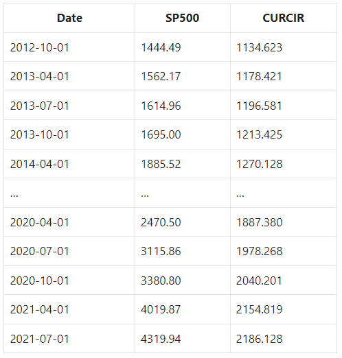
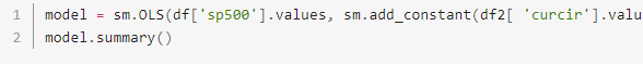
Use statsmodels to implement linear regression.

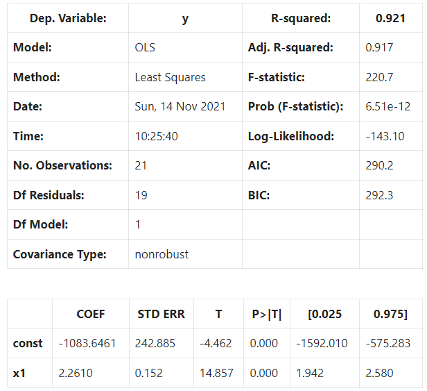
Our new linear model using the currency in circulation performs worse than our GDP model when comparing the r-squared value.

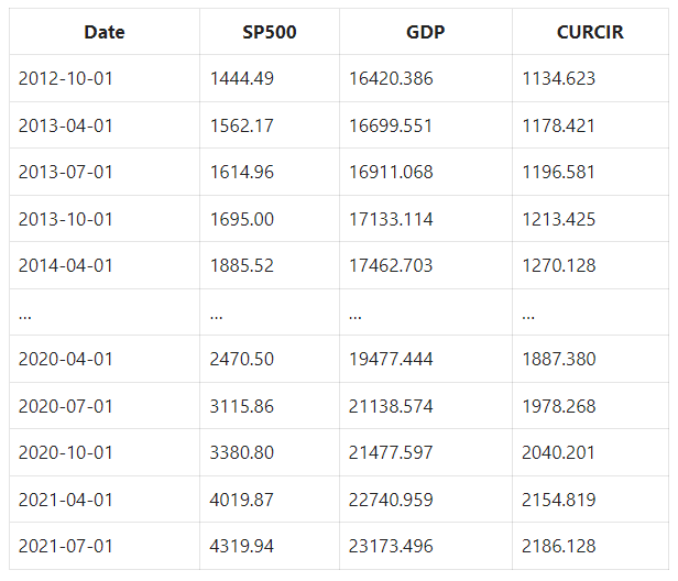
Multiple Linear Regression in Python

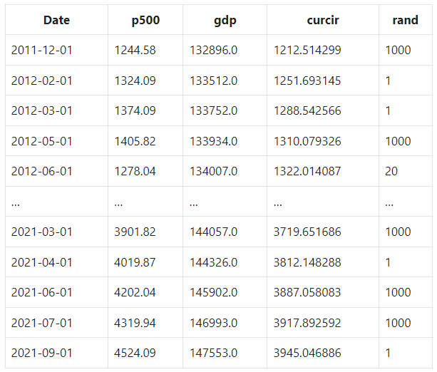
Let’s look at this data.

Here’s the code:

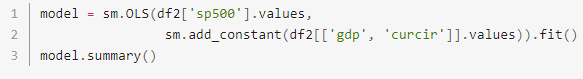
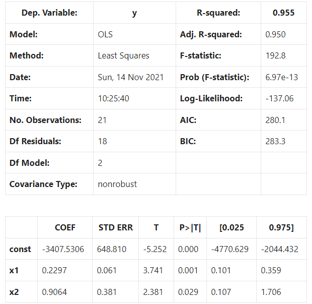
We can see that having two variables improved the model. 

Notice there’s one more coefficient in the model coefficients section in the regression model.

y = b_0 + b_1* X_1 + b_2 * X_2

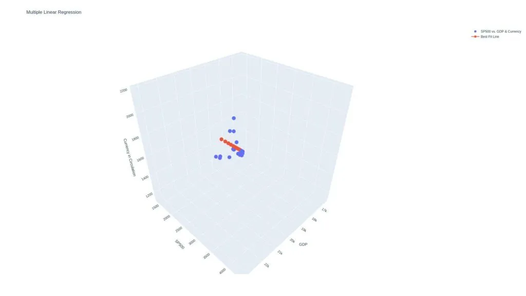
How do we visualize this?

Visualizing Multiple Linear Regression

Let’s create a multiple linear regression model 3d graph where the y-values are the s&p500, and the x and z values are GDP and currency in circulation, respectively.

Let’s add some random data to see how that affects our model. Let’s use a random one-dimensional array between 1 and 1000 in our multiple linear regression model.

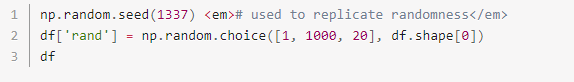
This is how it performs:

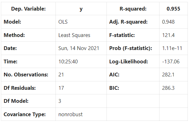
The r2 didn’t improve because we added random data.

But the rule of thumb is that if the p-value is 0.05 or lower, the coefficient and independent variable are said to be statistically significant.

So, if the p-value is small and the increase in r2 is large, add the variable to the input features; otherwise, discard.

Multicollinearity in Regression

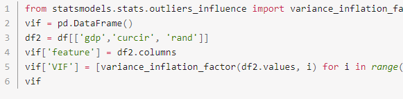
Multicollinearity is a statistical concept in which several independent model variables are correlated. This issue will result in less reliable statistical inferences. So we determine multicollinearity in our model data with Variance Inflation Factor (VIF).

Variance Inflation Factor

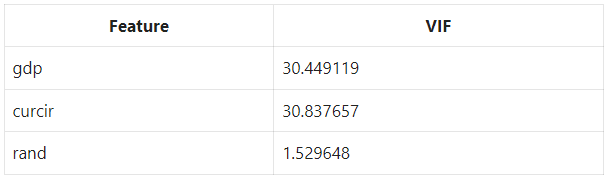
Note that:

• VIF of 1 indicates two variables are not correlated
• VIF greater than 1 and less than 5 indicates a moderate correlation
• VIF of 5 or above indicates a high correlation

Let’s use statsmodels.

Linear Regression in Machine Learning (Walk-Through)

Let’s use sklearn to create training data, and test data splits.

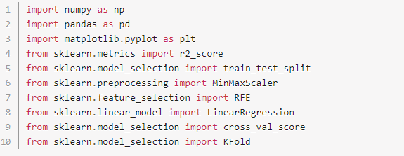
Required Imports

First, we need to get the required python modules:

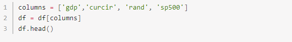
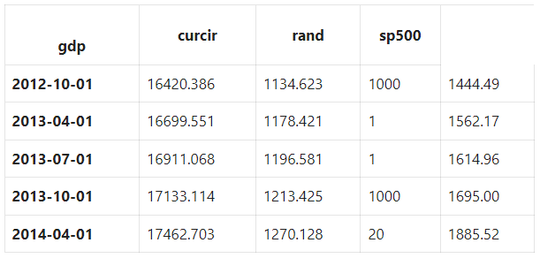
Then, organize the columns.

Scale and Normalize Data

For machine learning to work better, make sure that the features share the same scale and are normally distributed.

Let’s scale and standardize the variables between 0 and 1 using sklearn.preprocessing.MinMaxScaler.

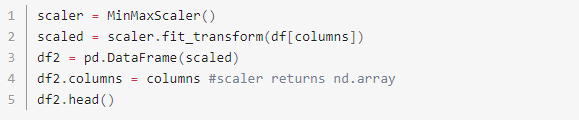
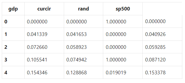
Notice that the features and targets are now scaled between zero and one.

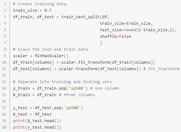
Split Data Into Train & Test Sets

Let’s separate the data into training and testing sets. 

We’ll train on 70% of the data and test on the remaining 30%. We’ll also scale our data properly instead of overfitting like we did above.

Now let’s fix our multicollinearity issue identified by VIF.

Recursive Feature Elimination

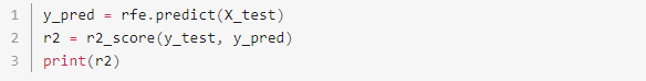
Let’s do this and see the output:

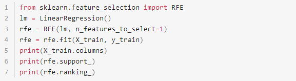
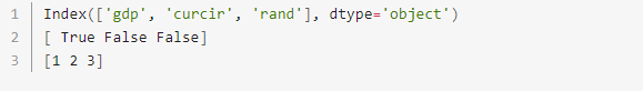
Notice that our n_features_to_select hyperparameter was set to one, causing RFE to select only GDP. We can also see the rankings are 1, 2, and 3 for GDP, currency in circulation, and our random variable, respectively.

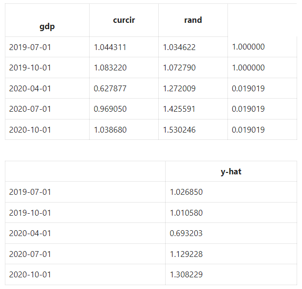
Create Linear Regression Model

Let’s create a linear regression model:

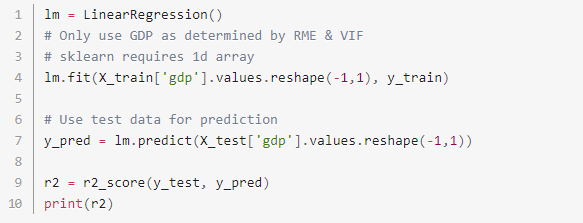
RFE selects the best features recursively and applies the LinearRegression model to it.

Cross-Validation Using K-Folds

Instead of splitting the data into one train set and one test set, we can slice the data into multiple periods. 

Let’s use four k-folds as an example. 

The first set will take the first 16 elements; the second will be the following 16 elements, the next 15 elements, and finally, our most recent 15 elements. Our array length is 62 and not evenly divisible by 4.

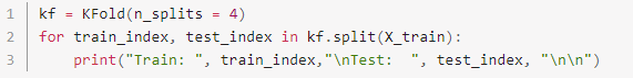
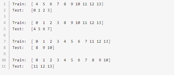
We now have four test and train data groups and can quickly estimate our r2 for each test group.

Analyze The Results

want to learn how to algo trade so you can remove all emotions from trading and automate it 100%? click below to join the free discord and then join the bootcamp to get started today.